
Non-Autoregressive Neural Machine Translation
최근의 neural network를 사용하는 machine translation 모델들은 기존의 통계적인 모델에 비해 좋은 성능을 내지만, decoder의 autoregressive한 특성 때문에 속도가 느린 단점이 있다.
본 연구에서는 non-autoregressive한 transformer를 소개한다.
Non-Autoregressive Decoding
Pros and cons of autoregressive decoding
기존의 machine translation에서 사용하는 autoregressive factorization은 몇가지 장점이 있다.
이는 사람이 word-by-word로 language를 만드는 방식과 일치하며, translation들의 분포를 효율적으로 구할 수 있다.
Autoregressive 모델들은 거대한 corpus에서 state-of-the-art의 성능을 발휘하며, 쉽게 학습할 수 있고, beam search 방식은 효과적으로 optimal에 가까운 translation들을 계산할 수 있다.
하지만, 단점들도 존재한다.
Decoder에서 각각의 step들이 parallel이 아닌 sequential하게 진행되기 때문에 transformer 같은 구조는 training 과정의 이점을 실제 inference에서는 사용할 수 없다.
Beam search는 beam size에 따라 성능이 감소될 수 있고, parallelism에 제약이 있다.
Towards non-autoregressive decoding
Naive한 방법은 encoder-decoder 모델에서 autoregressive한 연결을 제거하는 것이다.
이 모델의 출력 \(p_{NA}\)는 target sequence의 길이가 \(T\)라고 할 때, conditional distribution \(p_L\)와 함께 아래와 같이 계산할 수 있다.
\[p_{NA}(Y\mid X;\theta)=p_L(T\mid x_{1:T'};\theta)\cdot\Pi_{t=1}^Tp(y_t\mid x_{1:T'};\theta)\]즉, \(T'\)개의 source sequence가 주어졌을 때, target sequence의 길이 \(T\)를 예측하고, \(T\)개의 output \(y\)를 예측한다.
이 모델은 여전히 likelihood function을 가지고 있으며, 각각의 output에 대해 cross entropy loss를 계산해 학습시킬 수 있다.
하지만, 이 모델은 inference시에 parallel하게 계산을 해서 output을 만들 수 있다.
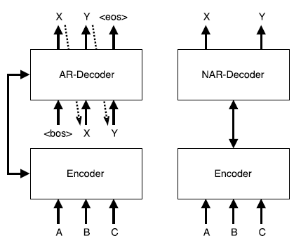
아래 그림은 autoregressive한 decoder와 non-autoregressive한 decoder의 차이를 보여준다.
The multimodality problem
위에서 소개한 naive한 방법은 conditional independence를 사용하기 때문에 좋은 성능을 내지 못한다.
각 token의 distribution \(p(y_t)\)는 source sequence인 \(X\)에만 의존한다.
이는 실제 target의 distribution에 접근하는 것을 어렵게 만든다.
직관적으로 생각하면, 여러 번역가들에게 각각 다른 번역가들이 말한 단어와는 연관성 없이 하나의 단어에 대한 번역을 시키는 것과 같다.
Conditional independence는 모델이 target sequence의 multimodal distribution을 학습하는 것을 어렵게 한다.
이런 문제를 multimodality problem이라고 이름 붙였고, 이를 해결하기 위한 기술을 소개한다.
The Non-Autoregressive Transformer(NAT)
본 연구에서는 NAT라는 새로운 모델로 machine translation task를 해결한다.
NAT는 전체 output을 parallel하게 생성할 수 있다.
NAT는 encoder stack, decoder stack, fertility predictor 그리고 translation predictor로 구성된다.
아래 그림은 NAT의 구조를 보여준다.
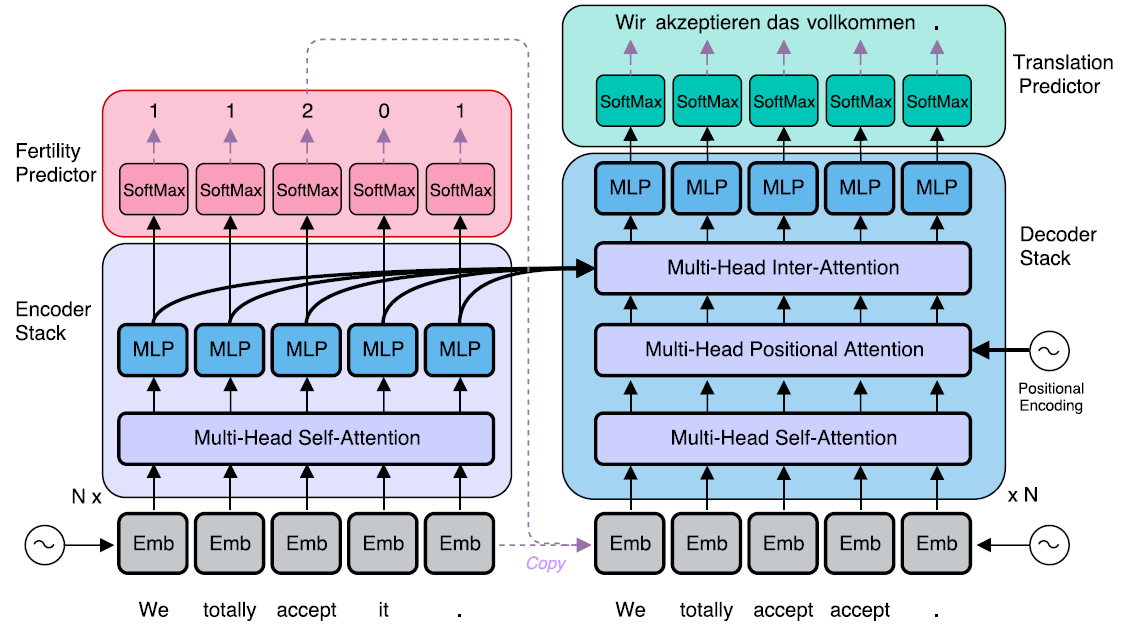
검은색 실선 화살표는 미분 가능, 보라색 점선 화살표는 미분 불가능을 의미한다.
Endoder와 decoder안의 각 sub layer들은 layer normalization과 residual 구조를 갖는다.
Encoder stack
Autoregressive transformer와 비슷하게 encoder와 decoder 모두 multi head attention과 feed forward network(MLP)로 구성된다.
RNN을 사용하지 않기 때문에 계산을 sequential하게 수행할 필요가 없고 non-autoregressive decoding을 가능하게 한다.
Encoder stack은 기존의 transformer의 encoder stack과 차이가 없다.
Decoder stack
Non-autoregressive하게 translation을 진행하고 decoding 과정을 parallel하게 만들기 위해 decoder stack을 다음과 같이 변형시켰다.
Decoder inputs
모든 word를 parallel하게 생성하기 위해서는 decoding을 시작하기 전에 target sequence의 길이를 알 필요가 있다.
기존의 transformer처럼 training시에는 time-shift된 target sequence를, inference시에는 이전 step에서 예측한 output 값을 첫번째 decoder layer의 input으로 사용하는 것은 불가능하다.
첫번째 layer의 input을 생략하거나 positional embedding만 사용하는 것은 성능을 크게 감소시킨다.
NAT에서는 encoder에서 사용했던 source sequence를 그대로 복사해서 decoding을 시작한다.
하지만 source와 target sequence는 길이가 다르기 때문에 다음 두가지 방법을 제안한다.
-
Copy source inputs uniformly
각 decoder의 input \(t\)는 \(Round(\frac{T't}{T})\) 번째 encoder의 input을 복사해 사용한다.
여기서, \(Round\)는 반올림을 의미한다.
이 방법은 source sequence를 일정한 속도로 복사하고, 예측한 target sequence의 길이 \(T\)만큼 output을 생성한다.
-
Copy sorcue inputs using fertilities
위의 그림에서 적용된 방법이며, encoder의 input을 decoder의 input으로 0번 이상 반복해서 복사한다.
여기서, encoder의 각 input들이 반복되는 회수를
fertility라고 한다.이 방법은 source sequence를 일정하지 않은 속도로 복사하고, target sequence의 길이는 source sequence의 fertility의 합이 된다.
Non casual self attention
Output에 대해 autoregressive factorization이라는 제약이 없기 때문에 decoding 과정에서 이전 time step들에서 이후의 time step들의 정보를 사용하는 것을 막을 필요가 없다.
즉, 기존의 transformer의 self attention에서 사용했던 mask를 사용할 필요가 없다.
본 연구에서는 그 대신, 각 position에서 자기 자신의 정보를 사용할 수 없도록 mask를 사용하는 것이 mask를 사용하지 않는 것 보다 성능을 향상시키는 사실을 발견했다.
Positional attention
각 decoder layer는 추가적인 positional attention 모듈을 갖는다.
이 모듈은 기존의 transformer에서 사용하는 attention 구조와 같다.
\[Attention(Q,K,V)=softmax(\frac{QK^T}{\sqrt{d_{model}}})\cdot V\]\(d_{model}\)은 모델의 hidden size이며, query와 key는 positional encoding 값이고 value는 decoder의 state 값이다.
이 방법은 positional 정보를 attention에 직접 통합시켜서 embedding에서만 positional encoding을 사용하는 것 보다 좀 더 강력한 위치 정보를 학습할 수 있게 한다.
Modeling fertility to tackle the multimodality problem
Latent variable \(z\)를 모델에 직접 추가함으로써 multimodality problem을 해결할 수 있다.
먼저, prior의 distribution으로 부터 \(z\)를 sampling한 후에 \(z\)를 사용해 non-autoregressive한 output을 생성한다.
\(z\)는 다음과 같은 특성들을 갖는다.
- 모델을 end-to-end 방식으로 학습시킬 때 필요하기 때문에 주어진 input-output 쌍을 통해 \(z\)를 추론하기 쉬워야 한다.
- \(z\)를 conditioning context에 더하는 것은 서로 다른 output들 사이에서 시간에 따른 상관관계를 최대한 고려해야 하므로, 각 output position에서 marginal probability를 남겨두는 것은 conditional independence를 만족시키는 것과 가까워진다.
- Output의 variation은 고려하지 않아야 하고, 그렇기 때문에 \(p(y\mid x,z)\)는 학습에 있어 trivial 하다.
NAT의 가장 중요한 특성 중 하나는 예측된 fertility에 기반해 encoder의 input을 복사할 때, 자연스럽게 정보를 갖고 있는 latent variable을 만들 수 있다는 것이다.
Source sequence \(X\)가 주어졌을 때, target sequence \(Y\)의 conditional probability는 아래와 같다.
\[p_{NA}(Y\mid X;\theta)=\sum_{f_1,...,f_{T'}\in \mathcal{F}}(\Pi_{t'=1}^{T'}p_F(f_{t'}\mid x_{1:T'};\theta))\cdot\Pi_{t=1}^Tp(y_t\mid x_1\{f_1\},...,x_{T'}\{f_{T'}\};\theta)\\ \mathcal{F}=\{f_1,...,f_{T'}\mid\sum_{t'=1}^{T'}f_{t'}=T,f_{t'}\in\mathbb{Z}^*\}\]여기서, \(\mathcal{F}\)는 fertility sequence들의 집합이다.
하나의 source word는 하나의 fertility를 가지며, 이를 모두 더하면 \(Y\)의 길이, \(T\)가 된다.
\(x\{f\}\)는 \(x\)가 \(f\)번 반복되는 것을 의미한다.
Fertility prediction
마지막 encoder layer의 output위에 one layer neural network와 softmax를 추가해서 각 position마다 독립적으로 fertility \(p_F(f_{t'}\mid x_{1:T'})\)를 계산한다.
이 방법은 fertility가 각 input word의 특성이면서 전체 문장의 context에 의존하도록 모델링한다.
Benefits of fertility
Fertility는 앞서 기술한 non-autoregressive한 machine translation을 위해 필요한 latent variable의 3가지 특성을 모두 만족한다.
-
Unsupervised training을 두개의 supervised training으로 효율적으로 축소시킴으로써 간단하고 빠른 inference 모델을 만들 수 있다.
-
Fertility를 latent variable로 사용하는 것은 output space의 자연스러운 factorization을 만들어 multimodality problem을 해결하는데에 큰 도움을 준다.
Source sequence가 주어지면, output의 distribution을 특정 fertility sequence와 일치하는 target sequence로 제한하는 것은 mode space를 크게 줄여준다.
Mode를 선택하는 것은 supervised 방식으로 학습될 수 있다.
-
Latent variable에 fertility와 reordering을 모두 포함시키는 것은 완전한 정렬의 확률을 제공한다.
이것은 latent variable이 주어졌을 때, decoding을 쉽게 만들며 encoder가 복잡한 모델링을 수행한다.
Fertility만 포함시키는 것은 encoder의 부담을 decoder에게 조금 덜어줄 수 있게 한다.
Fertility를 latent variable로 사용한다는 것은 translation의 길이를 분리해서 고려할 필요가 없다는 것을 의미한다.
또한, fertility는 sampling을 통해 다양한 translation을 가능하게 함으로써, decoding을 향상시킬 수 있다.
Translation predictor and the decoding process
Inference시에, 모델은 모든 latent fertility sequence에 대해 marginalization을 적용한 후에 가장 높은 확률의 word들로 translation을 수행한다.
Fertility sequence가 주어졌을 때, 최적의 translation은 각 position에서 독립적으로 local probability를 최대화시키는 것이다.
Source sequence와 fertility sequence가 주어졌을 때, 이러한 최적의 translation은 \(Y=G(x_{1:T'},f_{1:T'};\theta)\)로 정의한다.
하지만, 여전히 fertility space상에서 탐색과 marginalization을 추적하는 것은 불가능하기 때문에 space를 축소시키기 위한 3가지 휴리스틱한 decoding 알고리즘을 제안한다.
Argmax decoding
Fertility sequence도 conditionally independant factorization 방식으로 모델링 되기 때문에 다음과 같이 각 word마다 가장 높은 확률의 fertility를 선택함으로써 간단하게 최적의 translation을 추정할 수 있다. \(\hat{Y}_{argmax}=G(x_{1:T'},\hat{f}_{1:T'};\theta)\\ \hat{f}_{t'}=argmax_fp_F(f_{t'}\mid x_{1:T'};\theta)\)
Average decoding
또한, 아래와 같이 softmax의 expectation으로 각 fertility를 추정할 수 있다. \(\hat{Y}_{argmax}=G(x_{1:T'},\hat{f}_{1:T'};\theta)\\ \hat{f}_{t'}=Round(\sum_{f_{t'}=1}^LP_F(f_{t'}\mid x_{1:T'};\theta)f_{t'})\)
Noisy parallel decoding(NPD)
Target의 최적에 보다 정확하게 접근하는 방법은 fertility space에서 sampling을 하고, 각 fertility sequence의 최적의 translation을 계산하는 것이다.
그리고 autoregressive teacher를 사용해 최적의 translation을 아래와 같이 정의할 수 있다.
\[\hat{Y}_{NPD}=G(x_{1:T'},argmax_{f_{t'}\sim p_F}p_{AR}(G(x_{1:T'},f_{1:T'};\theta)\mid X;\theta);\theta)\]Decoding된 translation의 scoring function으로 autoregressive 모델을 사용할 때, decoder의 input이 모두 parallel하게 들어오기 때문에 빠른 속도로 실행될 수 있다.
NPD는 stochastic한 방법이고, 연산량을 sample의 크기 만큼 linear하게 증가시킨다.
하지만, 모든 sample들은 독립적으로 계산되고 scoring 되기 때문에 충분히 parallel한 계산이 가능하다면 하나의 translation을 계산하는 것 보다 2배의 연산으로 가능하다.
Training
NAT는 discrete한 sequential latent variable \(f_{1:T'}\)를 가진다.
이 variable의 conditional posterior 분포는 \(p(f_{1:T'}\mid x_{1:T'},y_{1:T};\theta)\)이고, 이에 근접하는 분포 \(q(f_{1:T'}\mid x_{1:T'},y_{1:T})\)를 사용한다.
이는 아래와 같이 전체 maximum likelihood에 대한 variational bound를 제공한다.
\[\mathcal{L}_{ML}=log\,p_{NA}(Y\mid X;\theta)=log\sum_{f_{1:T'}\in\mathcal{F}}p_F(f_{1:T'}\mid x_{1:T'};\theta)\cdotp(y_{1:T}\mid x_{1:T'},f_{1:T'};\theta)\\ \geq \mathbb{E}_{f_{1:T'}\sim q}[\underbrace{\sum_{t=1}^Tlog\,p(y_t\mid x_1\{f_1\},...,x_{T'}\{f_{T'}\};\theta)}_{Translation \,loss}+\underbrace{\sum_{t'=1}^{T'}log\,p_F(f_{t'}\mid x_{1:T'};\theta)}_{Fertility \,loss}]+H(q)\]분리되고, 고정된 fertility 모델로부터 정의되는 분포 \(q\)를 선택한다.
가능한 선택지는 external aligner의 output, 즉, 학습 데이터의 (source, target) 쌍의 fertility들과, autoregressive teacher 모델에서 사용된 attention으로 계산된 fertility들이라고 할 수 있다.
이 때, \(q\)는 deterministic하기 때문에 inference 과정을 단순화 시킬 수 있다.
결과적으로, loss function은 inference된 fertility를 사용해 supervised 방식으로 translation 모델 \(p\)와 fertility 모델 \(p_F\)를 동시에 학습시킬 수 있다.
Sequence level knowledge distillation
Latent fertility 모델은 대체로 non-augoregressive output의 분포가 multimodal target 분포에 근접하게 도와준다.
하지만 이는 학습 데이터의 non-determinism을 완전히 해결하지는 못한다.
많은 경우에, 하나의 fertility sequence에 대해 올바른 translation이 여러 개 존재한다.
그렇기 때문에, 추가적으로 sequence level knowled distillation을 적용해서 새로운 corpus를 만든다.
이 때, teacher 모델로써, autoregressive machine translation 모델을 기존의 데이터로 학습하고, 이 모델의 greedy output들을 non-autoregressive student 모델의 target으로 사용한다.
학습된 모델은 하나의 문장에 대해서 계속 같은 translation을 만들 것이므로, 이런 방법으로 얻은 target은 덜 noisy 하고, 더 deterministic 하다고 볼 수 있다.
하지만, 이런 target들은 원래의 데이터에 비해 품질이 낮을 수 있다.
Fine tuning
supervised fertility 모델은 전체 maximum likelihood loss를 translation과 fertility loss로 나눌 수 있게 해준다.
하지만 이것은 fertility predictor를 포함한 전체 모델을 end-to-end로 학습하는 것이 아니라, external aligner에 의해 제공되는 deterministic하고 근접한 inference 모델에 크게 의존한다.
그러므로, NAT가 수렴하도록 학습한 후에 fine tuning 과정을 제안한다.
추가적으로 teacher의 output 분포, 즉, word level knowledge distillation의 reverse KL divergence으로 이루어진 loss term을 아래와 같이 정의한다.
\[\mathcal{L}_{RKL}(f_{1:T'};\theta)=\sum_{t=1}^T\sum_{y_t}[log\,p_{AR}(y_t\mid \hat{y}_{1:t-1},x_{1:T'})\cdotp_{NA}(y_t\mid x_{1:T'},f_{1:T'};\theta)]\\ \hat{y}_{1:T}=G(x_{1:T'},f_{1:T'};\theta)\]이러한 loss는 매우 peaked한 student 모델의 output 분포에 있어 일반적인 cross entropy loss보다 유리하다.
그 후에, 기존 distillation loss의 weighted sum, inference된 fertility의 expectation, 그리고 external fertility model을 통해 전체 모델을 joint하게 학습시키며, 식은 아래와 같다.
\[\mathcal{L}_{FT}=\lambda(\underbrace{\mathbb{E}_{f_{1:T'}\sim p_F}[\mathcal{L}_{RKL}(f_{1:T'})-\mathcal{L}_{RKL}(\bar{f}_{1:T'})]}_{\mathcal{L}_{RL}}+\underbrace{\mathbb{E}_{f_{1:T'}\sim q}[\mathcal{L}_{RKL}(f_{1:T'})]}_{\mathcal{L}_{BP}})+(1-\lambda)\mathcal{L}_{KD}\]여기서, \(\bar{f}_{1:T'}\)는 \(\hat{f}_{t'}\)의 평균이다.
\(\mathcal{L}_{RL}\)은 미분이 불가능하기 때문에 gradient는 reinforcement learning으로 추정할 수 있으며, \(\mathcal{L}_{BP}\)는 일반적인 backpropagation으로 학습한다.
Leave a comment